A Binary (Max) Heap is a complete binary tree that maintains the Max Heap property.

Binary Heap is one possible data structure to model an efficient Priority Queue (PQ) Abstract Data Type (ADT). In a PQ, each element has a "priority" and an element with higher priority is served before an element with lower priority (ties are broken with standard First-In First-Out (FIFO) rule as with normal Queue). Try clicking ExtractMax() for a sample animation on extracting the max value of random Binary Heap above.

To focus the discussion scope, we design this visualization to show a Binary Max Heap that contains distinct integers only.

Click 'Next' (on the top right)/press 'Page Down' to advance this e-Lecture slide, use the drop down list/press 'Space' to jump to a specific slide, or Click 'X' (on the bottom right)/press 'Esc' to go to Exploration mode.

---

Remarks: By default, we show e-Lecture Mode for first time (or non logged-in) visitor.
Please login if you are a repeated visitor or register for an (optional) free account first.

Complete Binary Tree: Every level in the binary tree, except possibly the last/lowest level, is completely filled, and all vertices in the last level are as far left as possible.

Binary Max Heap property: The parent of each vertex - except the root - contains value greater than the value of that vertex. This is an easier-to-verify definition than the following alternative definition: The value of a vertex - except the leaf/leaves - must be greater than the value of its one (or two) child(ren).

---

Pro-tip: Since you are not logged-in, you may be a first time visitor who are not aware of the following keyboard shortcuts to navigate this e-Lecture mode: [PageDown] to advance to the next slide, [PageUp] to go back to the previous slide, [Esc] to toggle between this e-Lecture mode and exploration mode.

Priority Queue (PQ) Abstract Data Type (ADT) is similar to normal Queue ADT, but with these two major operations:

1. Enqueue(x): Put a new element (key) x into the PQ (in some order),
2. y = Dequeue(): Return an existing element y that has the highest priority (key) in the PQ and if ties, return the one that is inserted first, i.e. back to First-In First-Out (FIFO) behavior of a normal Queue

---

Another pro-tip: We designed this visualization and this e-Lecture mode to look good on 1366x768 resolution or larger (typical modern laptop resolution in 2017). We recommend using Google Chrome to access VisuAlgo. Go to full screen mode (F11) to enjoy this setup. However, you can use zoom-in (Ctrl +) or zoom-out (Ctrl -) to calibrate this.

Imagine: You are an Air Traffic Controller (ATC) working in the control tower of an airport.

You have scheduled aircraft X/Y to land in the next 3/6 minutes, respectively. Both have enough fuel for at least the next 15 minutes and both are just 2 minutes away from your airport. You observe that your airport runway is clear at the moment.

In case you do not know, aircraft can be instructed to fly in holding pattern near the airport until the designated landing time.

You have to attend the live lecture to figure out what happens next...

There will be two options presented to you and you will have to decide:

1. Raise AND wave your hand if you choose option A,
2. Raise your hand but do NOT wave it if you choose option B,

If none of the two options is reasonable for you, simply do nothing.

There are several potential usages of PQ ADT in real-life on top of what you have seen just now (only in live lecture).

Discussion: Can you mention a few other real-life situations where a PQ is needed?

We are able to implement this PQ ADT using (circular) array or Linked List but we will have slow (i.e. in O(N)) Enqueue or Dequeue operation.

Discussion: Why?

Now, let's view the visualisation of a (random) Binary (Max) Heap above. You should see a complete binary tree and all vertices except the root satisfy the Max Heap property (A[parent(i)] > A[i] — remember that we disallow duplicate integers here).

Quiz: Based on this Binary (Max) Heap property, where will the largest integer be located?

At one of the leaf
Can be anywhere
At the root

Submit

Important fact to memorize at this point: If we have a Binary Heap of N elements, its height will not be taller than O(log N) since we will store it as a complete binary tree.

Simple analysis: The size N of a full (more than just a complete) binary tree of height h is always N = 2^(h+1)-1, therefore h = log₂(N+1)-1 ~= log₂ N.

See example above with N = 7 = 2⁽²⁺¹⁾-1 or h = log₂(7+1)-1 = 2.

This fact is important in the analysis of all Binary Heap-related operations.

A complete binary tree can be stored efficiently as a compact array A as there is no gap between vertices of a complete binary tree/elements of a compact array. To simplify the navigation operations below, we use 1-based array. VisuAlgo displays the index of each vertex as a red label below each vertex. Read those indices in sorted order from 1 to N, then you will see the vertices of the complete binary tree from top to down, left to right.

This way, we can implement basic binary tree traversal operations with simple index manipulations (with help of bit shift manipulation):

1. parent(i) = i>>1, index i divided by 2 (integer division),
2. left(i) = i<<1, index i multiplied by 2,
3. right(i) = (i<<1)+1, index i multiplied by 2 and added by 1.

In this visualization, you can perform five (5) standard Binary (Max) Heap operations:

1. Insert(v) in O(log N)
2. ExtractMax() in O(log N)
3. Create(A) - O(N log N) version
4. Create(A) - O(N) version
5. HeapSort() - in O(N log N)

There are others possible Binary (Max) Heap operations, but currently we do not elaborate them for pedagogical reason in a certain NUS module.

Insert(v): Insertion of a new item v into a Binary Max Heap can only be done at the last index N plus 1 to maintain the compact array = complete binary tree property. However, the Max Heap property may still be violated. This operation then fixes Max Heap property from the insertion point upwards (if necessary) and stop when there is no more Max Heap property violation. Now try clicking Insert(v) several times to insert a few random v to the currently displayed Binary (Max Heap).

The fix Max Heap property upwards operation has no standard name. We call it ShiftUp but others may call it BubbleUp or IncreaseKey operation.

Do you understand why starting from the insertion point (index N+1) upwards (at most until the root) and swapping a vertex with its parent when there is a Max Heap property violation during insertion is always a correct strategy?

The time complexity of this Insert(v) operation is O(log N).

Discussion: Do you understand the derivation?

ExtractMax(): The reporting and then the deletion of the maximum element (the root) of a Binary Max Heap requires an existing element to replace the root, otherwise the Binary Max Heap (a single complete binary tree, or 林/Lín in Chinese/tree) becomes two disjoint subtrees (two copies of 木/mù in Chinese/wood). That element must be the last index N for the same reason: To maintain the compact array = complete binary tree property.

Because we promote a leaf vertex to the root vertex of a Binary Max Heap, it will very likely violates the Max Heap property. ExtractMax() operation then fixes Binary Max Heap property from the root downwards by comparing the current value with the its child/the larger of its two children (if necessary). Now try ExtractMax() on the currently displayed Binary (Max) Heap.

The fix Max Heap property downwards operation has no standard name. We call it ShiftDown but others may call it BubbleDown or Heapify operation.

Why if a vertex has two children, we have to check (and possibly swap) that vertex with the larger of its two children during the downwards fix of Max Heap property?

Why can't we just compare with the left (or right, if exists) vertex only?

The time complexity of this ExtractMax() operation is O(log N).

Discussion: Do you understand the derivation?

Up to here, we have a data structure that can implement the two major operations of Priority Queue (PQ) ADT efficiently:

1. For Enqueue(x), we can use Insert(x) in O(log N) time, and
2. For y = Dequeue(), we can use y = ExtractMax() in O(log N) time.

However, we can do a few more operations with Binary Heap.

Create(A): Creates a valid Binary (Max) Heap from an input array A of N integers (comma separated) into an initially empty Binary Max Heap.

There are two variants for this operations, one that is simpler but runs in O(N log N) and a more advanced technique that runs in O(N).

Pro tip: Try opening two copies of VisuAlgo on two browser windows. Execute different Create(A) versions on the worst case 'Sorted example' to see the somewhat dramatic differences of the two.

Create(A) - O(N log N): Simply insert (that is, by calling Insert(v) operation) all N integers of the input array into an initially empty Binary Max Heap one by one.

Analysis: This operation is clearly O(N log N) as we call O(log N) Insert(v) operation N times. Let's examine the 'Sorted example' which is one of the hard case of this operation (Now try the Hard Case - O(N log N) where we show a case where A=[1,2,3,4,5,6,7] -- please be patient as this example will take some time to complete). If we insert values in increasing order into an initially empty Binary Max Heap, then every insertion triggers a path from the insertion point (a new leaf) upwards to the root.

Create(A) - O(N): This faster version of Create(A) operation was invented by Robert W. Floyd in 1964. It takes advantage of the fact that a compact array = complete binary tree and all leaves (i.e. half of the vertices — see the next slide) are Binary Max Heap by default. This operation then fixes Binary Max Heap property (if necessary) only from the last internal vertex back to the root.

Analysis: A loose analysis gives another O(N/2 log N) = O(N log N) complexity but it is actually just O(2*N) = O(N) — details in the next few slides. Now try the Hard Case - O(N) on the same input array A=[1,2,3,4,5,6,7] and see that on the same hard case as with the previous slide (but not the one that generates maximum number of swaps), this operation is far superior than the O(N log N) version.

Simple proof on why half of Binary (Max) Heap of N (without loss of generality, let's assume that N is even) elements are leaves are as follows:

Suppose that the last leaf is at index N, then the parent of that last leaf is at index i = N/2 (remember this slide). The left child of vertex i+1, if exists (it actually does not exist), will be 2*(i+1) = 2*(N/2+1) = N+2, which exceeds index N (the last leaf) so index i+1 must also be a leaf vertex that has no child. As Binary Heap indexing is consecutive, basically indices [i+1 = N/2+1, i+2 = N/2+2, ..., N], or half of the vertices, are leaves.

First, we need to recall that the height of a full binary tree of size N is log₂ N.

Second, we need to realise that the cost to run shiftDown(i) operation is not the gross upper bound O(log N), but O(h) where h is the height of the subtree rooted at i.

Third, there are ceil(N/2^h+1) vertices at height h in a full binary tree.

On the example full binary tree above with N = 7 and h = 2, there are:
ceil(7/2⁰⁺¹) = 4 vertices: {44,35,26,17} at height h = 0,
ceil(7/2¹⁺¹) = 2 vertices: {62,53} at height h = 1, and
ceil(7/2²⁺¹) = 1 vertex: {71} at height h = 2.

Cost of Create(A), the O(N) version is thus:

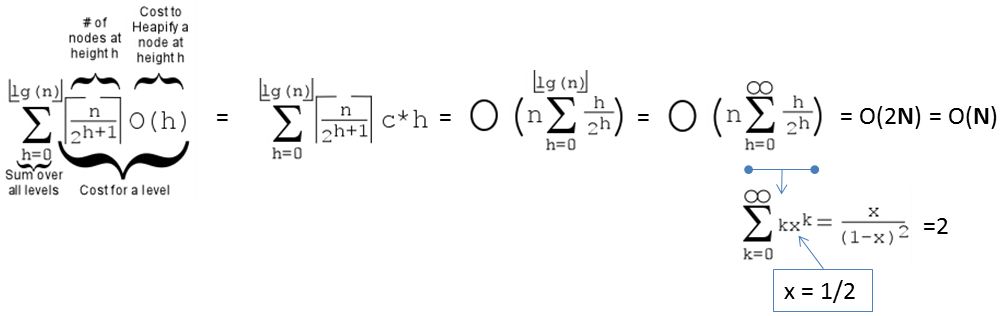
PS: If the formula is too complicated, a modern student can also use WolframAlpha instead.

HeapSort(): John William Joseph Williams invented HeapSort() algorithm in 1964, together with this Binary Heap data structure. HeapSort() operation (assuming the Binary Max Heap has been created in O(N)) is very easy. Simply call the O(log N) ExtractMax() operation N times. Now try HeapSort() on the currently displayed Binary (Max) Heap.

Simple Analysis: HeapSort() clearly runs in O(N log N) — an optimal comparison-based sorting algorithm.

Quiz: In worst case scenario, HeapSort() is asymptotically faster than...

Selection Sort
Insertion Sort
Merge Sort
Bubble Sort
Submit

Although HeapSort() runs in θ(N log N) time for all (best/average/worst) cases, is it really the best comparison-based sorting algorithm?

Discussion: How about caching performance of HeapSort()?

You have reached the end of the basic stuffs of this Binary (Max) Heap data structure and we encourage you to explore further in the Exploration Mode.

However, we still have a few more interesting Binary (Max) Heap challenges for you that are outlined in this section.

When you have cleared them all, we invite you to study more advanced algorithms that use Priority Queue as (one of) its underlying data structure, like Prim's MST algorithm, Dijkstra's SSSP algorithm, A* search algorithm (not in VisuAlgo yet), etc.

If you are looking for an implementation of Binary (Max) Heap to actually model a Priority Queue, then there is a good news.

C++ and Java already have built-in Priority Queue implementations that very likely use this data structure. They are C++ STL priority_queue (the default is a Max Priority Queue) and Java PriorityQueue (the default is a Min Priority Queue). However, the built-in implementation may not be suitable to do some PQ extended operations efficiently (details omitted for pedagogical reason in a certain NUS module).

Python heapq exists but its performance is rather slow. OCaml doesn't have built-in Priority Queue but we can use something else that is going to be mentioned in the other modules in VisuAlgo (the reason on why the details are omitted is the same as above).

PS: Heap Sort is likely used in C++ STL algorithm partial_sort.

---

Nevertheless, here is our implementation of BinaryHeapDemo.cpp.

For a few more interesting questions about this data structure, please practice on Binary Heap training module (no login is required).

However, for registered users, you should login and then go to the Main Training Page to officially clear this module and such achievement will be recorded in your user account.

We also have a few programming problems that somewhat requires the usage of this Binary Heap data structure: UVa 01203 - Argus and Kattis - numbertree.

Try them to consolidate and improve your understanding about this data structure. You are allowed to use C++ STL priority_queue or Java PriorityQueue if that simplifies your implementation.

As the action is being carried out, each step will be described in the status panel.

Control the animation with the player controls! Keyboard shortcuts are:

Left/right arrows: step backward/step forward
-/+: decrease/increase speed

Return to 'Exploration Mode' to start exploring!

Note that if you notice any bug in this visualization or if you want to request for a new visualization feature, do not hesitate to drop an email to the project leader: Dr Steven Halim via his email address: stevenhalim at gmail dot com.