Sorting is a very classic problem of reordering items (that can be compared, e.g. integers, floating-point numbers, strings, etc) of an array (or a list) in a certain order (increasing, non-decreasing, decreasing, non-increasing, lexicographical, etc).

There are many different sorting algorithms, each has its own advantages and limitations.

Sorting is commonly used as the introductory problem in various Computer Science classes to showcase a range of algorithmic ideas.

Without loss of generality, we assume that we will sort only Integers, not necessarily distinct, in non-decreasing order in this visualization. Try clicking Bubble Sort for a sample animation of sorting the list of 5 jumbled integers (with duplicate) above.

Click 'Next' (on the top right)/press 'Page Down' to advance this e-Lecture slide, use the drop down list/press 'Space' to jump to a specific slide, or Click 'X' (on the bottom right)/press 'Esc' to go to Exploration mode.

Remarks: By default, we show e-Lecture Mode for first time (or non logged-in) visitor.
Please login if you are a repeated visitor or register for an (optional) free account first.

Sorting problem has a variety of interesting algorithmic solutions that embody many Computer Science ideas:

1. Comparison versus non-comparison based strategies,
2. Iterative versus Recursive implementation,
3. Divide-and-Conquer paradigm (this or that),
4. Best/Worst/Average-case Time Complexity analysis,
5. Randomized Algorithms, etc.

Pro-tip: Since you are not logged-in, you may be a first time visitor who are not aware of the following keyboard shortcuts to navigate this e-Lecture mode: [PageDown] to advance to the next slide, [PageUp] to go back to the previous slide, [Esc] to toggle between this e-Lecture mode and exploration mode.

When an (integer) array A is sorted, many problems involving A become easy (or easier):

1. Searching for a specific value v in array A,
2. Finding the min/max or the k-th smallest/largest value in (static) array A,
3. Testing for uniqueness and deleting duplicates in array A,
4. Counting how many time a specific value v appear in array A,
5. Set intersection/union between array A and another sorted array B,
6. Finding a target pair x ∈ A and y ∈ A such that x+y equals to a target z, etc.

Discussion: In real-life classes, the instructor may elaborate more on these applications.

Another pro-tip: We designed this visualization and this e-Lecture mode to look good on 1366x768 resolution or larger (typical modern laptop resolution in 2017). We recommend using Google Chrome to access VisuAlgo. Go to full screen mode (F11) to enjoy this setup. However, you can use zoom-in (Ctrl +) or zoom-out (Ctrl -) to calibrate this.

There are two actions that you can do in this visualization.

The first action is about defining your own input, an array/a list that is:

1. Totally random,
2. Random but sorted (in ascending/descending order),
3. Random but nearly sorted (in ascending/descending order), or
4. Defined solely by yourself.

In Exploration mode, you can experiment with various sorting algorithms provided in this visualization to figure out their best and worst case inputs.

The second action is the most important one: Execute the active sorting algorithm by clicking "Sort" menu and then clicking "Go".

Remember that you can switch active algorithm by clicking the respective abbreviation on the top side of this visualization page.

Some sorting algorithms have certain additional options. You may toggle the options as you wish before clicking "Go". For example, in Bubble Sort (and Merge Sort), there is an option to also compute the inversion index of the input array (this is an advanced topic).

View the visualisation/animation of the chosen sorting algorithm here.

Without loss of generality, we only show Integers in this visualization and our objective is to sort them from the initial state into ascending order state.

At the top, you will see the list of commonly taught sorting algorithms in Computer Science classes. To activate each algorithm, select the abbreviation of respective algorithm name before clicking "Sort → Go".

To facilitate more diversity, we randomize the active algorithm upon each page load.

The first six algorithms are comparison-based sorting algorithms while the last two are not. We will discuss this idea midway through this e-Lecture.

The middle three algorithms are recursive sorting algorithms while the rest are usually implemented iteratively.

To save screen space, we abbreviate algorithm names into three characters each:

1. Comparison-based Sorting Algorithms:
   1. BUB - Bubble Sort,
   2. SEL - Selection Sort,
   3. INS - Insertion Sort,
   4. MER - Merge Sort (recursive implementation),
   5. QUI - Quick Sort (recursive implementation),
   6. R-Q - Random Quick Sort (recursive implementation).
2. Not Comparison-based Sorting Algorithms:
   1. COU - Counting Sort,
   2. RAD - Radix Sort.

We will discuss three comparison-based sorting algorithms in the next few slides:

1. Bubble Sort,
2. Selection Sort,
3. Insertion Sort.

They are called comparison-based as they compare pairs of elements of the array and decide whether to swap them or not.

These three sorting algorithms are the easiest to implement but also not the most efficient, as they run in O(N²).

Before we start with the discussion of various sorting algorithms, it may be a good idea to discuss the basics of asymptotic algorithm analysis, so that you can follow the discussions of the various O(N^2), O(N log N), and special O(N) sorting algorithms later.

This section can be skipped if you already know this topic.

You need to already understand/remember all these:
-. Logarithm and Exponentiation, e.g., log₂(1024) = 10, 2¹⁰ = 1024
-. Arithmetic progression, e.g., 1+2+3+4+…+10 = 10*11/2 = 55
-. Geometric progression, e.g., 1+2+4+8+..+1024 = 1*(1-2¹¹)/(1-2) = 2047
-. Linear/Quadratic/Cubic function, e.g., f1(x) = x+2, f2(x) = x²+x-1, f3(x) = x³+2x²-x+7
-. Ceiling, Floor, and Absolute function, e.g., ceil(3.1) = 4, floor(3.1) = 3, abs(-7) = 7

Analysis of Algorithm is a process to evaluate rigorously the resources (time and space) needed by an algorithm and represent the result of the evaluation with a (simple) formula.

The time/space requirement of an algorithm is also called the time/space complexity of the algorithm, respectively.

For this module, we focus more on time requirement of various sorting algorithms.

We can measure the actual running time of a program by using wall clock time or by inserting timing-measurement code into our program, e.g., see the code shown in SpeedTest.cpp|java|py.

However, actual running time is not meaningful when comparing two algorithms as they are possibly coded in different languages, using different data sets, or running on different computers.

Instead of measuring the actual timing, we count the # of operations (arithmetic, assignment, comparison, etc). This is a way to assess its efficiency as an algorithm's execution time is correlated to the # of operations that it requires.

See the code shown in SpeedTest.cpp|java|py and the comments (especially on how to get the final value of variable counter).

Knowing the (precise) number of operations required by the algorithm, we can state something like this: Algorithm X takes 2n² + 100n operations to solve problem of size n.

If the time t needed for one operation is known, then we can state that algorithm X takes (2n² + 100n)t time units to solve problem of size n.

However, time t is dependent on the factors mentioned earlier, e.g., different languages, compilers and computers, etc.

Therefore, instead of tying the analysis to actual time t, we can state that algorithm X takes time that is proportional to 2n² + 100n to solving problem of size n.

Asymptotic analysis is an analysis of algorithms that focuses on analyzing problems of large input size n, considers only the leading term of the formula, and ignores the coefficient of the leading term.

We choose the leading term because the lower order terms contribute lesser to the overall cost as the input grows larger, e.g., for f(n) = 2n² + 100n, we have:
f(1000) = 2*1000² + 100*1000 = 2.1M, vs
f(100000) = 2*100000² + 100*100000 = 20010M.
(notice that the lower order term 100n has lesser contribution).

Suppose two algorithms have 2n² and 30n² as the leading terms, respectively.

Although actual time will be different due to the different constants, the growth rates of the running time are the same.

Compared with another algorithm with leading term of n³, the difference in growth rate is a much more dominating factor.

Hence, we can drop the coefficient of leading term when studying algorithm complexity.

If algorithm A requires time proportional to f(n), we say that algorithm A is of the order of f(n).

We write that algorithm A has time complexity of O(f(n)), where f(n) is the growth rate function for algorithm A.

Mathematically, an algorithm A is of O(f(n)) if there exist a constant k and a positive integer n0 such that algorithm A requires no more than k*f(n) time units to solve a problem of size n ≥ n0, i.e., when the problem size is larger than n0 algorithm A is (always) bounded from above by this simple formula k*f(n).

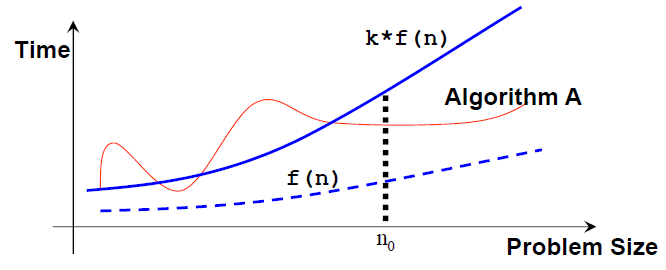
Note that: n0 and k are not unique and there can be many possible valid f(n).

In asymptotic analysis, a formula can be simplified to a single term with coefficient 1.

Such a term is called a growth term (rate of growth, order of growth, order of magnitude).

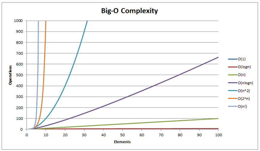
The most common growth terms can be ordered from fastest to slowest as follows
Note that many others are not shown (also see the visualization in the next slide):
O(1)/constant time < O(log n)/logarithmic time < O(n)/linear time <
O(n log n)/quasilinear time < O(n²)/quadratic time < O(n³)/cubic time <
O(2ⁿ)/exponential time < O(n!)/also-exponential time < ...

We will see three different growth rates O(n²), O(n log n), and O(n) throughout the remainder of this sorting module.

Given an array of N elements, Bubble Sort will:

1. Compare a pair of adjacent items (a, b),
2. Swap that pair if the items are out of order (in this case, when a > b),
3. Repeat Step 1 and 2 until we reach the end of array
   (the last pair is the (N-2)-th and (N-1)-th items as we use 0-based indexing),
4. By now, the largest item will be at the last position.
   We then reduce N by 1 and repeat Step 1 until we have N = 1.

Without further ado, let's try Bubble Sort on the small example array [29, 10, 14, 37, 14].

You should see a 'bubble-like' animation if you imagine the larger items 'bubble up' (actually 'float to the right side of the array').

Comparison and swap require time that is bounded by a constant, let's call it c.

There are two nested loops in (the standard) Bubble Sort.

The outer loop runs for exactly N iterations.
But the inner loop runs get shorter and shorter:

1. When i=0, (N−1) iterations (of comparisons and possibly swaps),
2. When i=1, (N−2) iterations,
   ...,
3. When i=(N−2), 1 iteration,
4. When i=(N−1), 0 iteration.

Thus, the total number of iterations = (N−1)+(N−2)+...+1+0 = N*(N−1)/2 (derivation).

Total time = c*N*(N−1)/2 = O(N^2).

Bubble Sort is actually inefficient with its O(N^2) time complexity. Imagine that we have N = 10⁵ numbers. Even if our computer is super fast and can compute 10⁸ operations in 1 second, Bubble Sort will need about 100 seconds to complete.

However, it can be terminated early, e.g. try Bubble Sort on the small sorted ascending example shown above [3, 6, 11, 25, 39] where it terminates in O(N) time.

The improvement idea is simple: If we go through the inner loop with no swapping at all, it means that the array is already sorted and we can stop Bubble Sort at that point.

Discussion: Although it makes Bubble Sort runs faster in general cases, this improvement idea does not change O(N^2) time complexity of Bubble Sort... Why?

Given an array of N items and L = 0, Selection Sort will:

1. Find the position X of the smallest item in the range of [L...N−1],
2. Swap X-th item with the L-th item,
3. Increase the lower-bound L by 1 and repeat Step 1 until L = N-2.

Without further ado, let's try Selection Sort on the same small example array [29, 10, 14, 37, 13].

Without loss of generality, we can also implement Selection Sort in reverse:
Find the position of the largest item Y and swap it with the last item.

void selectionSort(int a[], int N) {
  for (int L = 0; L <= N-2; ++L) { // O(N)
    int X = min_element(a+L, a+N) - a; // O(N)
    swap(a[X], a[L]); // O(1), X may be equal to L (no actual swap)
  }
}

Total: O(N²) — To be precise, it is similar to Bubble Sort analysis.

Quiz: How many (real) swaps are required to sort [29, 10, 14, 37, 13] by Selection Sort?

Insertion sort is similar to how most people arrange a hand of poker cards.

1. Start with one card in your hand,
2. Pick the next card and insert it into its proper sorted order,
3. Repeat previous step for all cards.

Without further ado, let's try Insertion Sort on the small example array [40, 13, 20, 8].

void insertionSort(int a[], int N) {
  for (int i = 1; i < N; ++i) { // O(N)
    int X = a[i]; // X is the item to be inserted
    int j = i-1;
    for (; j >= 0 && a[j] > X; --j) // can be fast or slow
      a[j+1] = a[j]; // make a place for X
    a[j+1] = X; // index j+1 is the insertion point
  }
}

The outer loop executes N−1 times, that's quite clear.

But the number of times the inner-loop is executed depends on the input:

1. In best-case scenario, the array is already sorted and (a[j] > X) is always false
   So no shifting of data is necessary and the inner loop runs in O(1),
2. In worst-case scenario, the array is reverse sorted and (a[j] > X) is always true
   Insertion always occur at the front of the array and the inner loop runs in O(N).

Thus, the best-case time is O(N × 1) = O(N) and the worst-case time is O(N × N) = O(N²).

Quiz: What is the complexity of Insertion Sort on any input array?

Ask your instructor if you are not clear on this or read similar remarks on this slide.

We will discuss two (+half) comparison-based sorting algorithms in the next few slides:

1. Merge Sort,
2. Quick Sort and its Randomized version (which only has one change).

These sorting algorithms are usually implemented recursively, use Divide and Conquer problem solving paradigm, and run in O(N log N) time for Merge Sort and O(N log N) time in expectation for Randomized Quick Sort.

PS: The the non-randomized version of Quick Sort runs in O(N²) though.

Given an array of N items, Merge Sort will:

1. Merge each pair of individual element (which is by default, sorted) into sorted arrays of 2 elements,
2. Merge each pair of sorted arrays of 2 elements into sorted arrays of 4 elements,
   Repeat the process...,
3. Final step: Merge 2 sorted arrays of N/2 elements (for simplicity of this discussion, we assume that N is even) to obtain a fully sorted array of N elements.

This is just the general idea and we need a few more details before we can discuss the true form of Merge Sort.

We will dissect this Merge Sort algorithm by first discussing its most important sub-routine: The O(N) merge.

Given two sorted array, A and B, of size N₁ and N₂, we can efficiently merge them into one larger combined sorted array of size N = N₁+N₂, in O(N) time.

This is achieved by simply comparing the front of the two arrays and take the smaller of the two at all times. However, this simple but fast O(N) merge sub-routine will need additional array to do this merging correctly. See the next slide.

void merge(int a[], int low, int mid, int high) {
  // subarray1 = a[low..mid], subarray2 = a[mid+1..high], both sorted
  int N = high-low+1;
  int b[N]; // discuss: why do we need a temporary array b?
  int left = low, right = mid+1, bIdx = 0;
  while (left <= mid && right <= high) // the merging
    b[bIdx++] = (a[left] <= a[right]) ? a[left++] : a[right++];
  while (left <= mid) b[bIdx++] = a[left++]; // leftover, if any
  while (right <= high) b[bIdx++] = a[right++]; // leftover, if any
  for (int k = 0; k < N; k++) a[low+k] = b[k]; // copy back
}

Try Merge Sort on the example array [1, 5, 19, 20, 2, 11, 15, 17] that have its first half already sorted [1, 5, 19, 20] and its second half also already sorted [2, 11, 15, 17]. Concentrate on the last merge of the Merge Sort algorithm.

Before we continue, let's talk about Divide and Conquer (abbreviated as D&C), a powerful problem solving paradigm.

Divide and Conquer algorithm solves (certain kind of) problem — like our sorting problem — in the following steps:

1. Divide step: Divide the large, original problem into smaller sub-problems and recursively solve the smaller sub-problems,
2. Conquer step: Combine the results of the smaller sub-problems to produce the result of the larger, original problem.

Merge Sort is a Divide and Conquer sorting algorithm.

The divide step is simple: Divide the current array into two halves (perfectly equal if N is even or one side is slightly greater by one element if N is odd) and then recursively sort the two halves.

The conquer step is the one that does the most work: Merge the two (sorted) halves to form a sorted array, using the merge sub-routine discussed earlier.

void mergeSort(int a[], int low, int high) {
  // the array to be sorted is a[low..high]
  if (low < high) { // base case: low >= high (0 or 1 item)
    int mid = (low+high) / 2;	
    mergeSort(a, low  , mid ); // divide into two halves
    mergeSort(a, mid+1, high); // then recursively sort them
    merge(a, low, mid, high); // conquer: the merge subroutine
  }
}

Please try Merge Sort on the example array [7, 2, 6, 3, 8, 4, 5] to see more details.

Contrary to what many other CS printed textbooks usually show (as textbooks are static), the actual execution of Merge Sort does not split to two subarrays level by level, but it will recursively sort the left subarray first before dealing with the right subarray.

That's it, on the example array [7, 2, 6, 3, 8, 4, 5], it will recurse to [7, 2, 6, 3], then [7, 2], then [7] (a single element, sorted by default), backtrack, recurse to [2] (sorted), backtrack, then finally merge [7, 2] into [2, 7], before it continue processing [6, 3] and so on.

In Merge Sort, the bulk of work is done in the conquer/merge step as the divide step does not really do anything (treated as O(1)).

When we call merge(a, low, mid, high), we process k = (high-low+1) items.
There will be at most k-1 comparisons.
There are k moves from original array a to temporary array b and another k moves back.
In total, number of operations inside merge sub-routine is < 3k-1 = O(k).

The important question is how many times this merge sub-routine is called?

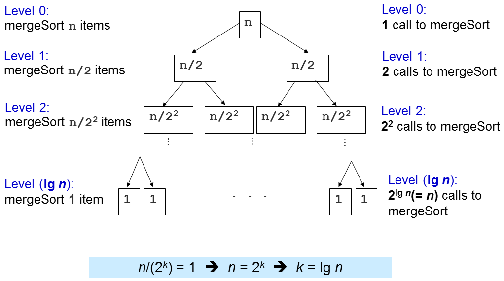
Level 1: 2^0=1 calls to merge() with N/2^1 items each, O(2^0 x 2 x N/2^1) = O(N)
Level 2: 2^1=2 calls to merge() with N/2^2 items each, O(2^1 x 2 x N/2^2) = O(N)
Level 3: 2^2=4 calls to merge() with N/2^3 items each, O(2^2 x 2 x N/2^3) = O(N)
...
Level (log N): 2^(log N-1) (or N/2) calls to merge() with N/2^log N (or 1) item each, O(N)

There are log N levels and in each level, we perform O(N) work, thus the overall time complexity is O(N log N). We will later see that this is an optimal (comparison-based) sorting algorithm, i.e. we cannot do better than this.

The most important good part of Merge Sort is its O(N log N) performance guarantee, regardless of the original ordering of the input. That's it, there is no adversary test case that can make Merge Sort runs longer than O(N log N) for any array of N elements.

Merge Sort is therefore very suitable to sort extremely large number of inputs as O(N log N) grows much slower than the O(N²) sorting algorithms that we have discussed earlier.

Merge Sort is also a stable sort algorithm. Discussion: Why?

There are however, several not-so-good parts of Merge Sort. First, it is actually not easy to implement from scratch (but we don't have to). Second, it requires additional O(N) storage during merging operation, thus not really memory efficient and not in-place. Btw, if you are interested to see what have been done to address these (classic) Merge Sort not-so-good parts, you can read this.

Quick Sort is another Divide and Conquer sorting algorithm (the other one discussed in this visualization page is Merge Sort).

We will see that this deterministic, non randomized version of Quick Sort can have bad time complexity of O(N²) on adversary input before continuing with the randomized and usable version later.

Divide step: Choose an item p (known as the pivot)
Then partition the items of a[i..j] into three parts: a[i..m-1], a[m], and a[m+1..j].
a[i..m-1] (possibly empty) contains items that are smaller than p.
a[m] is the pivot p, i.e. index m is the correct position for p in the sorted order of array a.
a[m+1..j] (possibly empty) contains items that are greater than or equal to p.
Then, recursively sort the two parts.

Conquer step: Don't be surprised... We do nothing :O!

If you compare this with Merge Sort, you will see that Quick Sort D&C steps are totally opposite with Merge Sort.

We will dissect this Quick Sort algorithm by first discussing its most important sub-routine: The O(N) partition (classic version).

To partition a[i..j], we first choose a[i] as the pivot p.

The remaining items (i.e. a[i+1..j]) are divided into 3 regions:

1. S1 = a[i+1..m] where items are < p,
2. S2 = a[m+1..k-1] where items are ≥ p, and
3. Unknown = a[k..j], where items are yet to be assigned to either S1 or S2.

Discussion: Why do we choose p = a[i]? Are there other choices?

Harder Discussion: Is it good to always put item(s) that is/are == p on S2 at all times?

Initially, both S1 and S2 regions are empty, i.e. all items excluding the designated pivot p are in the unknown region.

Then, for each item a[k] in the unknown region, we compare a[k] with p and decide one of the two cases:

1. If a[k] ≥ p, put a[k] into S2, or
2. Otherwise, put a[k] into S1.

These two cases are elaborated in the next two slides.

Lastly, we swap a[i] and a[m] to put pivot p right in the middle of S1 and S2.

int partition(int a[], int i, int j) {
  int p = a[i]; // p is the pivot
  int m = i; // S1 and S2 are initially empty
  for (int k = i+1; k <= j; k++) { // explore the unknown region
    if (a[k] < p) { // case 2
      m++;
      swap(a[k], a[m]); // C++ STL algorithm std::swap
    } // notice that we do nothing in case 1: a[k] >= p
  }
  swap(a[i], a[m]); // final step, swap pivot with a[m]
  return m; // return the index of pivot
}

void quickSort(int a[], int low, int high) {
  if (low < high) {
    int m = partition(a, low, high); // O(N)
    // a[low..high] ~> a[low..m–1], pivot, a[m+1..high]
    quickSort(a, low, m-1); // recursively sort left subarray
    // a[m] = pivot is already sorted after partition
    quickSort(a, m+1, high); // then sort right subarray
  }
}

Try Quick Sort on example array [27, 38, 12, 39, 27, 16]. We shall elaborate the first partition step as follows:
We set p = a[0] = 27.
We set a[1] = 38 as part of S2 so S1 = {} and S2 = {38}.
We swap a[1] = 38 with a[2] = 12 so S1 = {12} and S2 = {38}.
We set a[3] = 39 and later a[4] = 27 as part of S2 so S1 = {12} and S2 = {38,39,27}.
We swap a[2] = 38 with a[5] = 16 so S1 = {12,16} and S2 = {39,27,38}.
We swap p = a[0] = 27 with a[2] = 16 so S1 = {16,12}, p = {27}, and S2 = {39,27,38}.

After this, a[2] = 27 is guaranteed to be sorted and now Quick Sort recursively sorts the left side a[0..1] first and later recursively sorts the right side a[3..5].

First, we analyze the cost of one call of partition.

Inside partition(a, i, j), there is only a single for-loop that iterates through (j-i) times. As j can be as big as N-1 and i can be as low as 0, then the time complexity of partition is O(N).

Similar to Merge Sort analysis, the time complexity of Quick Sort is then dependent on the number of times partition(a, i, j) is called.

When the array a is already in ascending order, like the example above, Quick Sort will set p = a[0] = 5, and will return m = 0, thereby making S1 region empty and S2 region: Everything else other than the pivot (N-1 items).

Try Quick Sort on example input array [5, 18, 23, 39, 44, 50].

On such worst case input scenario, this is what happens:

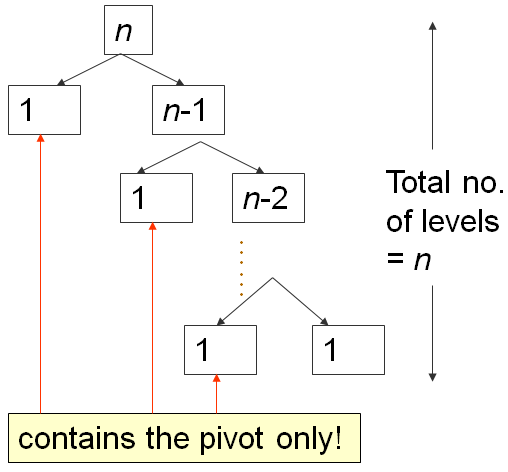
The first partition takes O(N) time, splits a into 0, 1, N-1 items, then recurse right.
The second one takes O(N-1) time, splits a into 0, 1, N-2 items, then recurse right again.
...
Until the last, N-th partition splits a into 0, 1, 1 item, and Quick Sort recursion stops.

This is the classic N+(N-1)+(N-2)+...+1 pattern, which is O(N²), similar analysis as the one in this slide...

The best case scenario of Quick Sort occurs when partition always splits the array into two equal halves, like Merge Sort.

When that happens, the depth of recursion is only O(log N).

As each level takes O(N) comparisons, the time complexity is O(N log N).

Try Quick Sort on this hand-crafted example input array [4, 1, 3, 2, 6, 5, 7].
In practice, this is rare, thus we need to devise a better way: Randomized Quick Sort.

Same as Quick Sort except just before executing the partition algorithm, it randomly select the pivot between a[i..j] instead of always choosing a[i] (or any other fixed index between [i..j]) deterministically.

Try Random Quick Sort on this large and somewhat random example array.

Mini exercise: Implement the idea above to the implementation shown in this slide!

It will take about 1 hour lecture to properly explain why this randomized version of Quick Sort has expected time complexity of O(N log N) on any input array of N elements.

In this e-Lecture, we will assume that it is true.

If you need non formal explanation: Just imagine that on randomized version of Quick Sort that randomizes the pivot selection, we will not always get extremely bad split of 0 (empty), 1 (pivot), and N-1 other items. This combination of lucky (half-pivot-half), somewhat lucky, somewhat unlucky, and extremely unlucky (empty, pivot, the rest) yields an average time complexity of O(N log N).

Discussion: Actually the phrase "any input array" above is not fully true. There is actually a way to make the randomized version of Quick Sort as currently presented in this VisuAlgo page still runs in O(N²). How?

We will discuss two non comparison-based sorting algorithms in the next few slides:

1. Counting Sort,
2. Radix Sort.

These sorting algorithms can be faster than the lower bound of comparison-based sorting algorithm of Ω(N log N) by not comparing the items of the array.

It is known (also not proven in this visualization as it will take another 1 hour lecture to do so) that all comparison-based sorting algorithms have a lower bound time complexity of Ω(N log N).

Thus, any comparison-based sorting algorithm with worst-case complexity O(N log N), like Merge Sort is considered an optimal algorithm, i.e. we cannot do better than that.

However, we can achieve faster sorting algorithm — i.e. in O(N) — if certain assumptions of the input array exist and thus we can avoid comparing the items to determine the sorted order.

Assumption: If the items to be sorted are Integers with small range, we can count the frequency of occurrence of each Integer (in that small range) and then loop through that small range to output the items in sorted order.

Try Counting Sort on the example array above where all Integers are within [1..9], thus we just need to count how many times Integer 1 appears, Integer 2 appears, ..., Integer 9 appears, and then loop through 1 to 9 to print out x copies of Integer y if frequency[y] = x.

The time complexity is O(N) to count the frequencies and O(N+k) to print out the output in sorted order where k is the range of the input Integers, which is 9-1+1 = 9 in this example. The time complexity of Counting Sort is thus O(N+k), which is O(N) if k is small.

We will not be able to do the counting part of Counting Sort when k is relatively big due to memory limitation, as we need to store frequencies of those k integers.

Assumption: If the items to be sorted are Integers with large range but of few digits, we can combine Counting Sort idea with Radix Sort to achieve the linear time complexity.

In Radix Sort, we treat each item to be sorted as a string of w digits (we pad Integers that have less than w digits with leading zeroes if necessary).

For the least significant (rightmost) digit to the most significant digit (leftmost), we pass through the N items and put them according to the active digit into 10 Queues (one for each digit [0..9]), which is like a modified Counting Sort as this one preserves stability. Then we re-concatenate the groups again for subsequent iteration.

Try Radix Sort on the example array above for clearer explanation.

Notice that we only perform O(w × (N+k)) iterations. In this example, w = 4 and k = 10.

There are a few other properties that can be used to differentiate sorting algorithms on top of whether they are comparison or non-comparison, recursive or iterative.

In this section, we will talk about in-place versus not in-place, stable versus not stable, and caching performance of sorting algorithms.

A sorting algorithm is said to be an in-place sorting algorithm if it requires only a constant amount (i.e. O(1)) of extra space during the sorting process. That's it, a few, constant number of extra variables is OK but we are not allowed to have variables that has variable length depending on the input size N.

Merge Sort (the classic version), due to its merge sub-routine that requires additional temporary array of size N, is not in-place.

Discussion: How about Bubble Sort, Selection Sort, Insertion Sort, Quick Sort (randomized or not), Counting Sort, and Radix Sort. Which ones are in-place?

A sorting algorithm is called stable if the relative order of elements with the same key value is preserved by the algorithm after sorting is performed.

Example application of stable sort: Assume that we have student names that have been sorted in alphabetical order. Now, if this list is sorted again by tutorial group number (recall that one tutorial group usually has many students), a stable sort algorithm would ensure that all students in the same tutorial group still appear in alphabetical order of their names.

Discussion: Which of the sorting algorithms discussed in this e-Lecture are stable?
Try sorting array A = {3, 4a, 2, 4b, 1}, i.e. there are two copies of 4 (4a first, then 4b).

We are nearing the end of this e-Lecture.

Time for a few simple questions.

Quiz: Which of these algorithms run in O(N log N) on any input array of size N?

Quiz: Which of these algorithms has worst case time complexity of Θ(N^2) for sorting N integers?

Θ is a tight time complexity analysis where the best case Ω and the worst case big-O analysis match.

We have reached the end of sorting e-Lecture.

However, there are two other sorting algorithms in VisuAlgo that are embedded in other data structures: Heap Sort and Balanced BST Sort. We will discuss them when you go through the e-Lecture of those two data structures.

Actually, the C++ source code for many of these basic sorting algorithms are already scattered throughout these e-Lecture slides. For other programming languages, you can translate the given C++ source code to the other programming language.

Usually, sorting is just a small part in problem solving process and nowadays, most of programming languages have their own sorting functions so we don't really have to re-code them unless absolutely necessary.

In C++, you can use std::sort, std::stable_sort, or std::partial_sort in STL algorithm.
In Java, you can use Collections.sort.
In Python, you can use sort.
In OCaml, you can use List.sort compare list_name.

If the comparison function is problem-specific, we may need to supply additional comparison function to those built-in sorting routines.

Note: Please Sign up/Login before attempting the training!

Test your understanding here!

Now that you have reached the end of this e-Lecture, do you think sorting problem is just as simple as calling built-in sort routine?

Try these online judge problems to find out more:
Kattis - mjehuric
Kattis - sortofsorting, or
Kattis - sidewayssorting

This is not the end of the topic of sorting. When you explore other topics in VisuAlgo, you will realise that sorting is a pre-processing step for many other advanced algorithms for harder problems, e.g. as the pre-processing step for Kruskal's algorithm, creatively used in Suffix Array data structure, etc.

As the action is being carried out, each step will be described in the status panel.

Control the animation with the player controls! Keyboard shortcuts are:

Return to 'Exploration Mode' to start exploring!

Note that if you notice any bug in this visualization or if you want to request for a new visualization feature, do not hesitate to drop an email to the project leader: Dr Steven Halim via his email address: stevenhalim at gmail dot com.